Significant ozone loss during winter 2019/2020 observed from ground based microwave radiometer
2026-05-21 - Kiruna, Sweden
Richard Johansson
Todays talk
- Scope of the study and instruments
- How chemical ozone loss happens
- Significance of NH winter 2019/2020
- Data and processing
- MIRA2 and MLS comparison
- Chemically induced ozone depletion
- Conclusions and future
Scope of study
- Compare ozone obtained with MIRA2 with satellite observations
- Use MIRA2 ozone observations to calculate chemical ozone depletion of winter 2019/2020
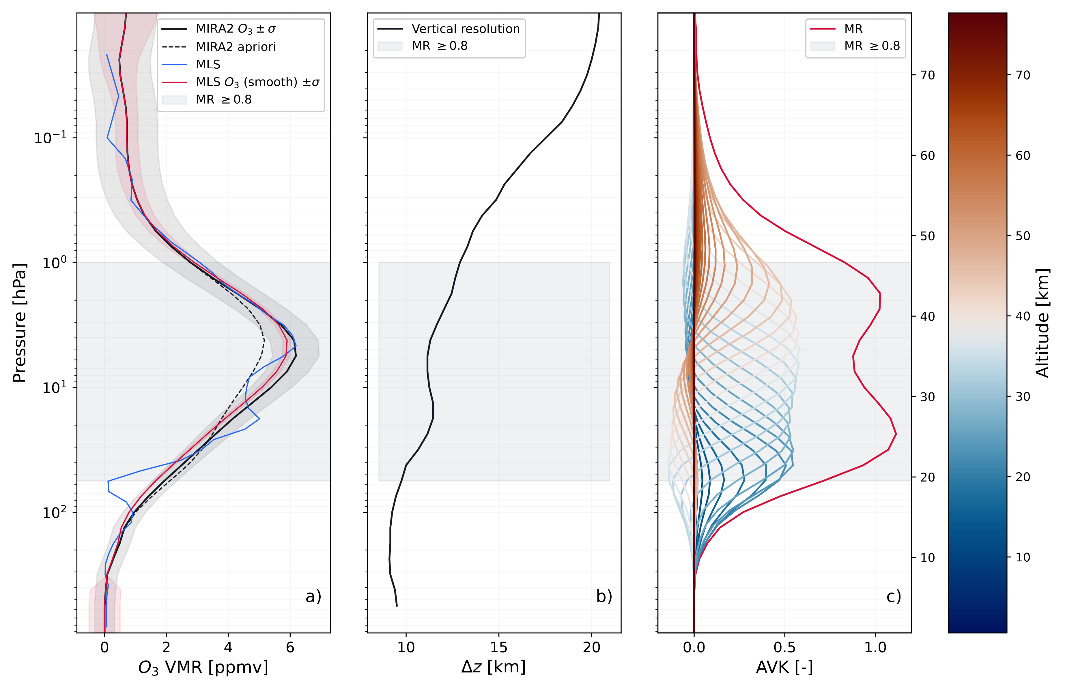
MIRA2 and MLS
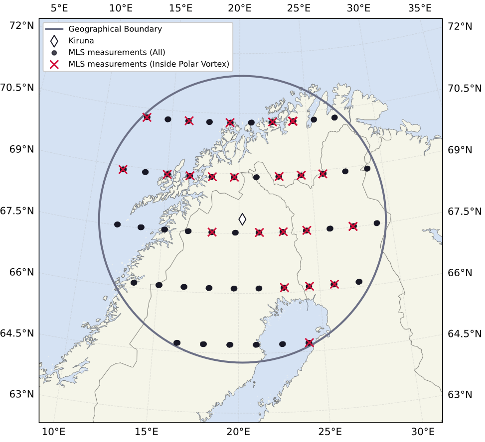
- Ground-based MWR situated at the Swedish Institute of Space Physics in Kiruna
- Measure ozone from 273.05 GHz emission line
- Continous measurement since 2014
- MLS onboard Aura satellite
- MLS measures atmospheric trace gases, including ozone.
- Covers altitudes from 5 to 120 km.
- Provides near-global coverage every three days.
- Serves as a widely used reference dataset for atmospheric research.
- Continous measurements since 2004
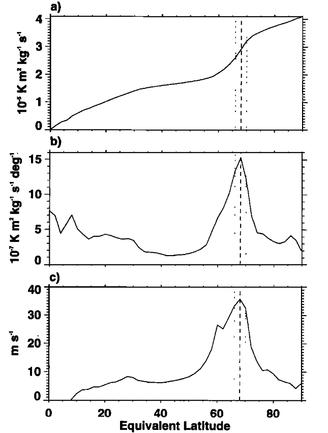
Polar vortex
PSC Chemistry & Ozone Depletion
Winter 2019/2020
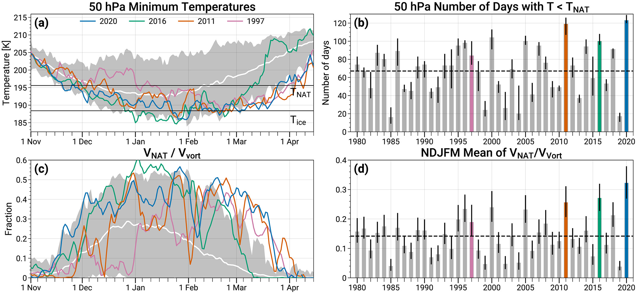
Figure 3: Daily 50-hPa minimum temperatures north of 40$^\circ$N (a) and the fraction of the lower-stratospheric vortex below the NAT PSC threshold, $V_{\mathrm{NAT}}/V_{\mathrm{vort}}$ (c). Annual summaries show the number of days with $T < T_{\mathrm{NAT}}$ (b) and the November--March mean $V_{\mathrm{NAT}}/V_{\mathrm{vort}}$ (d). Black lines in (a) indicate approximate NAT and ice PSC thresholds; whiskers in (b,d) show the range from a $\pm 1$ K uncertainty in $T_{\mathrm{NAT}}$ .
Data selection
MLS processing
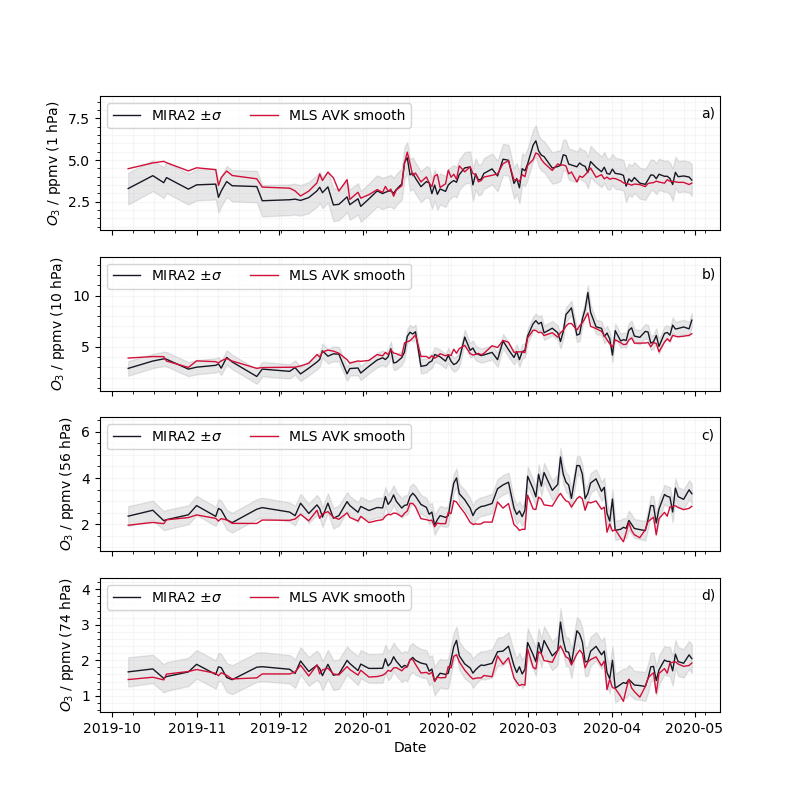
MIRA2 and MLS timeseries
Vertical coordinate
- Evaluated on isentropic surface of potential temperature:
$\theta = T\begin{pmatrix}\dfrac{P_0}{P}\end{pmatrix}^{R/c_p}$
- Easier comparison with previous studies
- Easier air-parcel tracking
Change in ozone
- Calculated from daily means
- Measurements obtained within the polar vortex
- Change from two sources:
- Dynamics
- Chemistry
$\Delta O_3 = O_{3P} - O_{3M}$
Dynamics: $O_{3P}$
Dynamics + Chemistry: $O_{3M}$
Tracer relation
- Use chemically inert for tracking dynamics
- Nitrous oxide ($N_2O$)
- Workflow to calculate $\Delta O_3$:
- Get $N_2O$ / $O_3$ reference function
- Calculate $O_{3P}$ from $N_2O$
- Get $O_{3M}$ from MIRA2
- Calculate chemically induced loss $\Delta O_3$
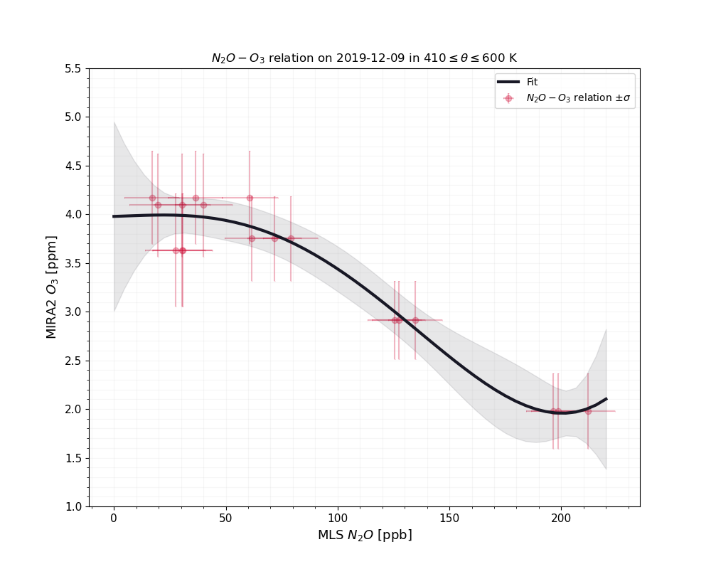
Figure 7: $N_2O-O_3$ reference function (black) with observations from MLS and MIRA2 (red scatter). Data is obtained from 2019-12-09 within the polar vortex and between 410 and 600 $K$
Ozone loss during winter 2019/2020
- $\Delta O_3$ evaluated from early December 2019 to mid April 2020
- Evaluated on isentropic surface of 475 K
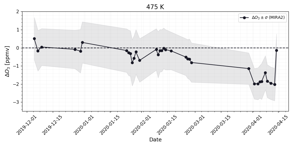
Figure 8: Cumulative chemically induced ozone loss ($\Delta O_3=O_{3P} - O_{3M}$) at the 475 K isentropic level derived from MIRA2 observations. Shaded region indicate total retrieval uncertainty $\sigma$ .
- Maximum loss observed early April 2020
- Chemical induced loss of $2.04\pm 0.91$ ppmv
Conclusions
- MIRA2 and MLS agree well
- Observed ozone loss ($2.04 \pm 0.91$) from MIRA2 also agree with previous studies:
- MLS studies show maximum loss of $2.8$ ppm at 460 K
- Transport and chemistry models show loss of $2.3-2.6$ ppm
Future work
- Under peer review
- First comments are positive
- Revision and publication during summer
- Guest instrument: WASPAM
- Measure $\mathrm{H_2O}$ at 22.235 GHz
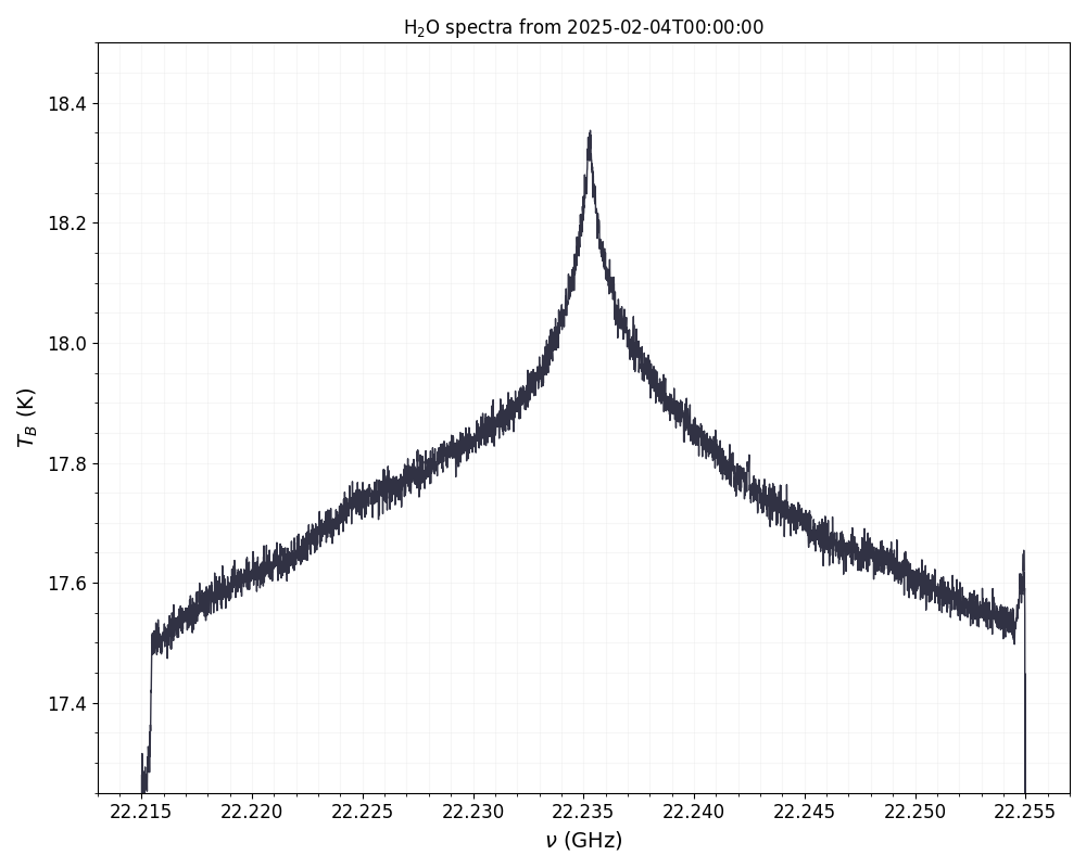
Figure 9: WASPAM spectra of water vapour line centered at 22.235 GHz. Spectra is obtained from 10h integration centered at midnight 2025-02-04